
Update: Based on questions I’ve received, I added the Misc Notes section to the end of this post.
Continuing with our #FunctionFriday series, today we’re going to explore how to use the IF, SEARCH, and ISNUMBER functions together to find text (aka a string) inside other text for classification purpose. What Excel really needs is a CONTAINS function, so we don’t have to do these mental acrobats. But, for now, this is what we have to work with.
To illustrate it, I’ll use an example from a chart I include in client dashboards** where they use the AddThis or ShareThis WordPress plugin. The data from these plugins populates to your Google Analytics account. BUT the data is such a red-hot mess, you have to do some cleanup to get it all into nice, neat buckets.
If you’d like to include this report in your own reports, you can use this custom report I created. (If you get a 404 error, it’s because you’re not logged in to Google Analytics. You have to be logged in to apply the report to your Google Analytics profile, aka view.)
**If you want to become a beast at building dashboards using the Google Analytics API, my online course will take you there.
Download Excel Workbook
If you’d like to follow along, you can download the Excel workbook I used in this demo.
The Functions du Jour
IF Function
The IF function is the Swiss Army knife for marketers, especially when you’re building out dynamic dashboards. With the IF function you start with a test — e.g., if A3=B2, if A3>=100, if A3=”organic”, etc. — and then you specify what you want to return if the condition is true and what you want to return if the value is false. But the fun doesn’t stop there; you can actually embed IF functions inside of IF functions. And that’s what we’re going to do in this tutorial.
It follows the following syntax:
IF(logical_test, [value_if_true], [value_if_false])
SEARCH Function
The SEARCH function is a tricky little bugger. It returns the position of whatever character you search for. And if you enter a string of characters, it will return the position of the first character in the matching string. So if you searched for cheese in the string string cheese, it would return the value of 8.
The SEARCH function follows the following syntax:
SEARCH( substring, string, [start_position] )
substring: Pure, unbridled geek speak that means whatever text you’re searching for, e.g., cheese.
string: Typically the cell this text string is in, though you could enter text as long as you flank it with quotation marks. (I almost always use a cell reference.)
start_position: This is optional. I usually only use it when I’m searching for forward slashes in URLs and want to start searching after the http(s)://. You can check out an example in this post that describes how to extract domains from URLs.
Now, if you put a string inside a SEARCH function, it will look for that string exactly. But you can also throw the asterisk wildcard in there for a really good time, which tells Excel to flag any string that even contains the text you’re searching for. So going back to our string cheese example, if I searched for cheese, it would return FALSE; if I searched for *cheese*, it would return TRUE.
ISNUMBER Function
The ISNUMBER function simply tells you if the cell you’re referencing is a value (or number). It’s Boolean, meaning it returns either a value of TRUE or FALSE.
It follows the following syntax:
ISNUMBER(value)
Pro Tip
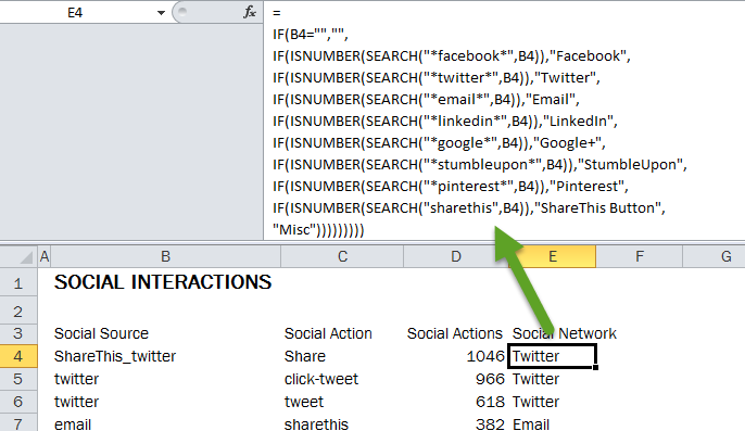
When dealing with a more complicated IF function, like you’ll see below, a good strategy is to break it into separate lines in the formula bar. To add a line break on a PC, use Alt-Enter; on a Mac, use Control-Option-Enter. I break my IF functions into different lines if I have more than three nested IFs. Here’s what it looks like for the formula we’ll use:
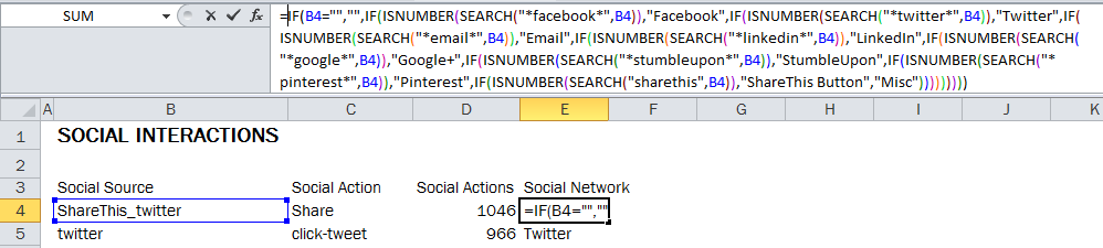
If you fat finger something in your formula, it’s really easy to see using this strategy because the IF functions won’t line up. When I’m finished, I just collapse the formula bar back to size by clicking-and-dragging the bottom of it.
Here’s what that same formula would look like if I didn’t use line breaks:
Putting It All Together
Okay, so here’s how we’re going to use them in concert. The Google Analytics custom report we’re using in this demo uses two dimensions: Social Source and Social Action and one metric, Social Actions. It’s a flat report, which, betedubs, is perfect for pivot tables. (Again, you should have data in this report if you use the ShareThis or AddThis plugin on WordPress.) But you could use this same strategy with any marketing data that you have to bucket based on snippets of text inside of strings.
If the formula in cell E4 could talk in plain English (wouldn’t that be nice?), here’s what it would say: “Hey, Excel, check out cell B4. If you see the string facebook anywhere in there, ISNUMBER will return a value of TRUE because you’ll return a number telling me the position of where the string I’m searching for. I don’t actually care about where that string is, only that it returns a number. If it does (IOW, it returns a value of TRUE), return the string Facebook; if it’s false, look for the next sting (i.e., twitter) and return Twitter … Rinse and repeat until you’ve cycled through all of the criteria. And if you don’t find facebook, twitter, email, linkedin, google, stumbleupon, pinterest, or sharethis, just call it Misc.” (Obviously, switch out sharethis for addthis if you’re using that plugin.)
Misc Notes
Difference Between SEARCH and FIND
Someone asked me about using the FIND function on Facebook instead of SEARCH. I rarely use the FIND function because it’s not as flexible as SEARCH. For one, it’s case sensitive. I can only remember one time using it because I needed to differentiate between cases. A much bigger liability is you can’t use it for partial matches because it doesn’t support Excel’s wildcard characters (* and ?).
Extracting Text Instead Of Categorizing It
So what if you didn’t want to match exact or partial text for the purpose of categorizing it like I have in this post with the help of the IF and ISNUMBER functions? What if, instead, you wanted to extract it instead? Then you would use the SEARCH function with the LEFT, RIGHT, and/or MID functions. I demonstrate how to do that in this tutorial on pulling domain names from a list of URLs. (I use this technique in conjunction with pivot tables in just about all competitive analysis I do because it allows me to group backlinks by domain.)
Hi Annie, I am trying to extract pricing information from a column called Product Description (col C). In column A is the Category and in Col B is the Sub-Category. The challenge is that there could be anywhere from 1 to a 100 prices embedded in a Col C. All prices are prepended with ||. My objective is to convert the data set into a Pivot table. For this I need the numbers in their own cells. However, I don’t want to create new columns after Col C. Is there a way to extract a price stick it in a newly row underneath while simultaneously copying the data from Col A and B? Btw, I like your site.
Sorry, Josh. I can’t even begin to understand what exactly you need here. If you want to include a link to a sample file with dummy data and clear instructions of what you need in that file, I can take a look at it.
Here is the link to my dummy data http://1drv.ms/1mcw7EC
It can definitely be done, but you’ll need a macro. The guy who does all of my macros is Justin Taylor. You can contact him to see if he can write it for you:
jtaylormade05@yahoo.com.
Hi Annie,
I have a list of street addresses from a marketing list with approximately 3000 records that I want to match to what I already have in my master list of over 25000 records. I used a MATCH formula to find a partial match of the first 8 characters. However, when I spot checked the results for streets with an apostrophe as the second character, I encountered a problem. For example, the record in my master list is 100 O’Malley Court. The record on the new marketing list is 100 OMalley Ct., or 100 O Malley Ct. Since, as a general rule, I’m looking for a partial match of the first 8 characters, what can I do to have Excel recognize either of the two address variations with what I have in my master list?
Thanks,
Tim
You can use the * and ? wildcard characters. But if you use too many, you’re going to get unfavorable results. But putting a ? between the O and Malley should capture all of those possibilities.
Hi Annie,
I watched your video on extracting the domain from a url and it was very helpful. It is ALMOST what i need help on. I have about 20 urls that have keys and values within. For example in the URL there would be : http://…………….;control=running;subcontrol=marathon;subcontrol2=triathalon…..
The problem i am having is that the URL’s have different values for control, subcontrol, subcontrol2 ect….Because it is in the middle of the URL i have having trouble extracting it.
I need to be able to write one function to call each URL’s value into their respective column. Let me know if you can help!
Ally
Hi Ally,
I’m not following. Are you trying to extract each of the values for your parameters into different columns?
Hi Annie, I watched your VLOOKUP and MATCH videos but can’t seem to get a partial text match to work. Most of the companies in my report have slight variations (“LLC” “LLC.” etc) that won’t work with any exact match search . How can I use the wildcard * to look up the first 4 characters in Column A and search the Column C Array to see if they exist?
Or any other ideas so all of these Column A companies show existing in Column B?
https://docs.google.com/spreadsheets/d/10vGm5G3PIB8U4sYYLX4mh0cMtSOLAmd81C5y2RVmZaY/edit?usp=sharing
Thanks much!
You’d have to use an array formula. Here’s what it would look like in your Google Spreadsheet: https://docs.google.com/spreadsheets/d/1fmbIZ9njpYfa1E2TiFVYHHvHQ1KQPc8QiLnnCzg3jNY/edit#gid=0.
Hi Annie
I’ve been searching high and low for a simialr answer and it looks as though I have found it based on your Google Doc you provided Al.
The one big problem I have is how can I implement this in Excel. Basically I would like to implement the same ARRAYFUNCTION on the GoogleDoc you provided Al in Excel to return the same results before implementing it on my own spreadsheet.
Basically I’m wanting to do a partial text match and then set a flag of Yes/No True False etc.
I have tried various way to implement the same in Excel but don’t seem to be getting anywhere
I would be very greatful if you could provide feedback
Please ignore I’m being stupid I have just downloaded document as excel file
doh!!!!
excelent blog
Man apologies
I’m spamming you now. Once I downloaded and open the sheet it changed the last two items from No to Yes.
So same question does still apply above
Sorry, Gordon, I’m not following what you need.
If you want to know more about “Searching for text in Excel”, check this link ……..
http://www.exceltip.com/excel-editing/searching-for-text-in-microsoft-excel.html
Brilliant stuff Annie……this works for me…..many thanks 🙂
My pleasure, Sharad!
Hi,
I am looking for help and I think it’s related. I need a “web-search-like-functionality” on a spread sheet.
Thus this is what I need / want it to do automatically:
If I use filters in a spreadsheet to search for a key word using Text Filters -> Contains I will type “x” and click ok. The result will be the spreadsheet will filter the spreadsheet looking for cells in that column containing “x”. Simple.
Can I make a cell available on this spreadsheet for my people to type the “x” in (like a search field on a web page), hit a macro button (or something similar) to filter the spreadsheet automatically for them after typing the desired “x” and hitting enter or alternatively a Macro button. Then the result will be that they see a much more reduced list with only the “x” contained in the spreadsheet?
I hope it makes sense, and I would appreciate any help you might be able to give.
Hello I have Question
I have data contain serial numbers and inside it conain dealer code for example
And i have matrix contain subdealer code and full name of this code
Please advise which the formulas can use taking into your kind consideration that i have soluation if the matrix contain one cell and write on it the subdealer code as
=replace(a1;search(b2;a1;1);len(b2);1)
And i have another question
How i can add validation on many cell and contain droplist to prevent duplicate
I know to prevent the duplicate but without use droplist as
In data validation write
=countif($a$1:$a$10;a1)=1
Please advise
Thank you very much
Hi Annie,
I hope you can help me as I’ve being trying hard to find a resolution to my issue. I am trying a value that has a partial match to a value that I put in a cell and then list the first 5 ‘partial match’ values in a column:
– In cell C1 i put in a formula that looks at cell A1 where I have typed in ‘Access’.
– Then excel looks in a separate sheet in column A to find all occurrences where ‘Access’ is contained in values in that column; such as ‘Access Control’, ‘Access Services’, Access Control Services’, ‘Controlled Access Services’.
– The formula then takes the first value from column B and puts this in the formula cell (C1).
– I then need to have all other partial matches put below in cells C2-C5.
– If there are not 5 matches a just need a blank cell
Hope you can help
Thanks
Kevin
Thanks so much for this! Helped me with exactly what I needed. Love the site!
Sorry for the horrifically late response! I didn’t realize I wasn’t receiving comment alerts. :/ But great! So glad I could help!
Hi Annie,
Thank you for this tutorial, it really helped. Is it possible to add another formula within the ‘result’? ie instead of final value of “Facebook”, can I add formula “((J2-Z2)*0.5))”. Every other step works for me except adding an additional formula for the output.
Thanks
Mike
This helps a great deal, but I’m still not quite there with what I need to do. I’m looking for “RUSH” in a text string in cells B4 through B419, and asking Excel to put “RUSH” or “Standard” in cells L4 through L419.
I tried the following array formula:
{=IF(ISNUMBER(SEARCH(RUSH,B4:B419)), “RUSH”, “Standard”)}
But it returned “Standard” in all instances.
Can you help me? I’m feeling a bit dim on this.
Sorry for the horrifically late response! I didn’t realize I wasn’t receiving comment alerts. :/ I assume you’ve gotten your answer by now.
use the formula:
=IF(ISNUMBER(SEARCH(“RUSH”,B4)),”RUSH”,”STANDARD”)
Annie, this is just awesome. Thank you very much, I’ve just used this to sort through 700 lines of key phrases for an adwords campaign and auto allocate them to ad groups. Ok this time around it probably took me as long to write and correct the formula… but next time…
Great stuff thank you.
John
Sorry for the horrifically late response! I didn’t realize I wasn’t receiving comment alerts. :/
But this is always my favorite kind of feedback to hear! So glad it helped – and will help even more next time! 🙂
I am trying to find a particular text within a cell and once found, want to extract a value next to the search text into another cell.
Eg. My cell A1 contains text “‘Client Number mismatch | Market : | Country : | PNR : XXXXXX | Invoice : 9999999 | Eticket : | Client Group ‘ABCD’ doesn’t match with PNR Client Group ‘EFGH’.”
In A2, I want to populate value EFGH when the search in A1 encounters “PNR Client Group”. (EFGH is the value coming after “PNR Client Group” in this example).
Hope you can help !! Thanks !!
It really help but it has some limitation of above tutorial Condition – If a string contains None, One No-One, everyone,anyone etc we need to count all these from a string then it will return irrelevant results.
Annie, great explainaniton and the formulae i’ve built works well apart from when using a wild card that has a numeric in it when i have more than 9 terms in the formuale. eg
IF(ISNUMBER(SEARCH(“*PERIOD 1*”,C3599)),”Jan”,
IF(ISNUMBER(SEARCH(“*PERIOD 2*”,C3599)),”Feb”,
IF(ISNUMBER(SEARCH(“*PERIOD 3*”,C3599)),”Mar”,
IF(ISNUMBER(SEARCH(“*PERIOD 4*”,C3599)),”Apr”,
IF(ISNUMBER(SEARCH(“*PERIOD 5*”,C3599)),”May”,
IF(ISNUMBER(SEARCH(“*PERIOD 6*”,C3599)),”Jun”,
IF(ISNUMBER(SEARCH(“*PERIOD 7*”,C3599)),”Jul”,
IF(ISNUMBER(SEARCH(“*PERIOD 8*”,C3599)),”Aug”,
IF(ISNUMBER(SEARCH(“*PERIOD 9*”,C3599)),”Sep”,
IF(ISNUMBER(SEARCH(“*PERIOD 10*”,C3599)),”Oct”,
IF(ISNUMBER(SEARCH(“*PERIOD 11*”,C3599)),”Nov”,
IF(ISNUMBER(SEARCH(“*PERIOD 12*”,C3599)),”Dec”,))))))))))))
returns “Jan” for Periods 10, 11 & 12. any suggections for fixing?
Regards,
Danny
found the answer, have reordered the Jan search to be the final term so teh whol formulea works now.
I’m sorry. I’m not understanding your question. :/
Hi Annie, great article!
I’m looking for a variation of this function, and hoping you can help.
I want to search (or count) multiple variables within a cell, as opposed to just looking for one.
So for example, below i have five random characters, and i’m looking for the letters (a,e,i,o,u,v,m), the counts or search result would look like this:
abcde = true (2)
bcddr = false (0)
bcvwr = true (1)
bamvg = true (2)
xrwpt = false (0)
mxrpm = true (2)
aaaai = true (5)
vvvvf = true (4)
axaxa = true (3)
zzzzz = false (0)
Can you help me recreate this in formula form?
Sorry. I couldn’t follow what you’re trying to do. Maybe toss it out on an Excel forum so you get a quicker answer?
I am trying to sift through a client’s twitter archive to harvest the #s that they used for their future use and reference. Is it possible to do a search and extract any word that begins with a #?
This will give you what you want w/o the #:
=RIGHT(IFERROR(MID(A1,SEARCH(“#”,A1),LEN(A1)-SEARCH(” “,A1,SEARCH(“#”,A1)+1)),RIGHT(A1,LEN(A1)-SEARCH(” #”,A1))),LEN(IFERROR(MID(A1,SEARCH(“#”,A1),LEN(A1)-SEARCH(” “,A1,SEARCH(“#”,A1)+1)),RIGHT(A1,LEN(A1)-SEARCH(” #”,A1))))-1)
If you want the #, go with this:
=RIGHT(IFERROR(MID(A1,SEARCH(“#”,A1),LEN(A1)-SEARCH(” “,A1,SEARCH(“#”,A1)+1)),RIGHT(A1,LEN(A1)-SEARCH(” #”,A1))),LEN(A1)-1)
Of course, update the A1s in the formula to whatever cell your data starts in, and then just apply the formula to the rest of the column by double-clicking the bottom-right corner of the cell in which you enter the formula.
My query is..
If in Sheet1, the value of cell A1 is AZ-1956045-abbyy-123456 and in Sheet2, the value of cell A1 is 1956045-abbyy-123456.
Is there a possible way to return the value 1956045-abbyy-123456 (cell A1, in Sheet2) next to the cell A1 in Sheet 1 i.e., in cell A2
I might be misunderstanding your question, but couldn’t you just reference =Sheet2!A1 in A2 of Sheet1 and then drag it down the column?
In cell A2 of Sheet 1, use this formula:
=Sheet2!A1